
A Deep Insight into Marketing Mix Modeling - Definition, Methodology, Comparison, Techniques
By Sam Nguyen

Drive 20-40% of your revenue with Avada
Marketing Mix Modeling, also known as MMM, is a familiar term with any business owners. MMM refers to a method used with an attempt to measure how much marketing inputs influence sales or marketing share. Once business people know how much each marketing input contributes to sales, they will draw out the correct budget for their businesses to spend on each marketing input.
Marketing Mix Modeling technique is so since it will decide the success and failure of a product launch or service promotion in the market. Therefore, every business is willing to spend time and money building an efficient marketing mix.
That’s why we have this post covering a brief definition and a deep insight into marketing mix modeling.
Let’s dive in!
What is the marketing mix modeling?
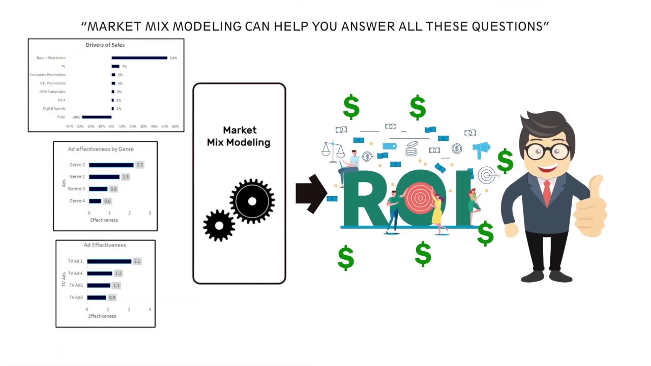
Marketing mix modeling (or MMM in short) is a statistical technique designed to evaluate the impact of various marketing inputs on sales. In this way, businesses know how to guess how future sets of tactics work. Marketing mix modeling helps users fulfill the following goals:
-
Maximizing advertising mix and promotional tactics to get higher sales revenue or profit. With a proper marketing mix model, businesses can ascertain the effect of each input related to return or investment. It means that a marketing input having higher ROI is more profitable as a medium than one with a lower ROI number.
-
Making the right business decisions in measuring the effectiveness of various marketing initiatives because they know exactly what and how marketing activities make changes to the business metrics.
First launched by econometricians a long time ago, MMM was first in use for consumer packaged goods, which resulted from the fact that producers of those goods could access the accurate sales data and marketing support materials. Then, when the data is more available, computer and technology develop more increasingly, and pressure to measure and optimize marketing is getting higher, MMM turns into a marketing tool that is applied more and more often over the world.
Today, the marketing mix modeling technique is considered a reliable marketing tool that any marketing company should have. In terms of the digital media context, MMM is sometimes referred to as attribution modeling. However, they are not the same. Such differences will be presented in the later parts of this post.
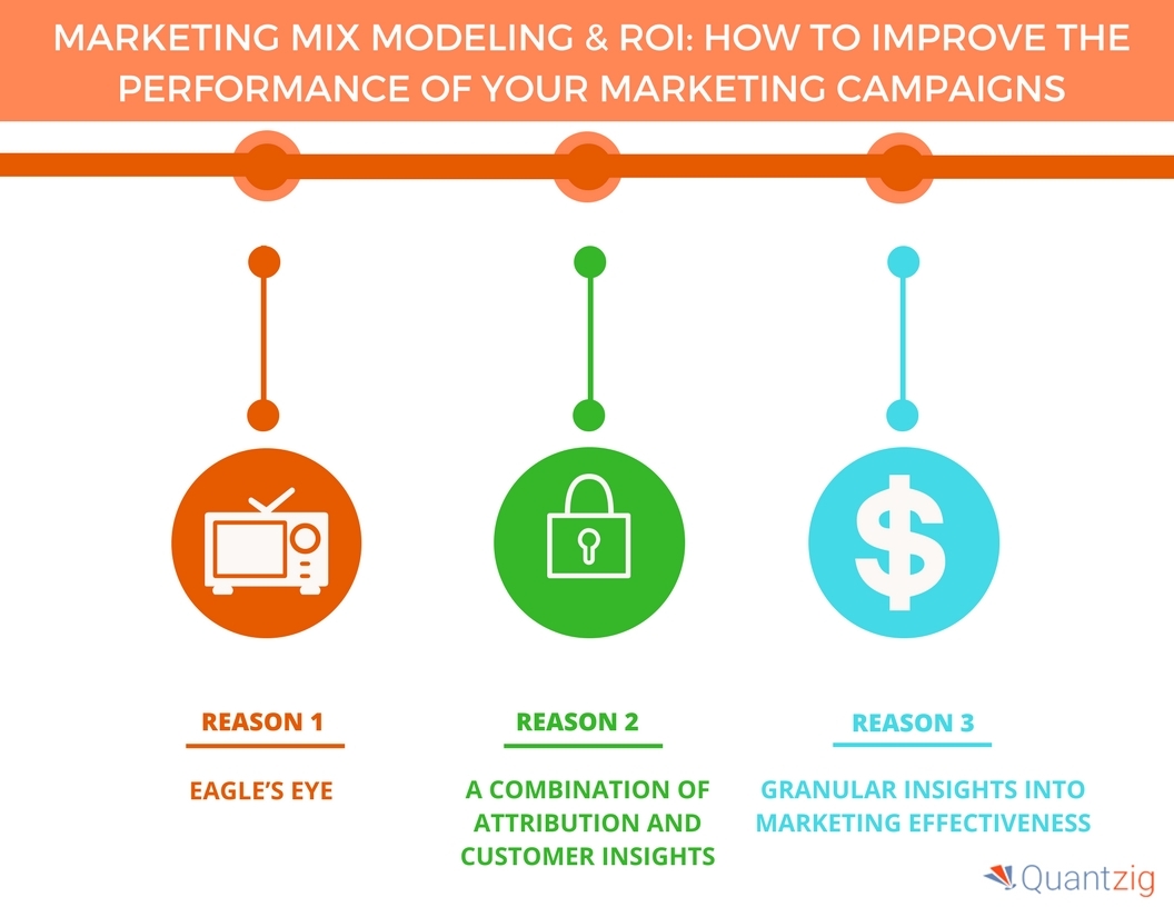
Marketing Mix Modeling is so important because it provides the benefits below:
-
Better plan on spending marketing budgets: Having a good MMM method, businesses can know which marketing channel is the best for themselves (TV, broadcast, radio, print, and more). From that, they can easily reach the marketing objectives and get maximum returns.
-
Better advertising campaigns: When having MMM, businesses better understand relevant markets that indirectly suggest optimal spend levels in marketing channels to prevent themselves from saturation.
-
Business scenario testing: Planned marketing activities are used as a kind of evidence to guess business metrics and test possible business scenarios.
Read more:
Marketing mix modeling methodology
This part will cover all common concepts you need to know while understanding marketing mix modeling.
Multi-Linear Regression
As you know, Multi-Linear Regression’s principle decides the marketing mix modeling. Therefore, it is the first thing you need to know when understanding MMM. When it comes to Multi-Linear Regression, IDVs and DVs can be:
-
The dependent variables (DVs): Sales or Market share
-
The independent variables (IDVs): price, distribution, TV spendings, outdoor campaign spendings, newspaper and magazine spendings, below-the-line promotional spendings, or consumer promotions data, etc.
Input for MMM can now include digital spending, website visitors, etc. It is because the digital medium is becoming more and more common due to its ability to increase brand exposure and brand awareness.
The related equation formed between the dependent variables and predictors can be either linear or non-linear. Whether it is linear or not bases on the relation between the dependent variable and multiple marketing inputs. For example, a TV advertisement is a specific variable that has a non-linear relationship with sales. It means that when TV GRP is increased, sales will not be impacted directly in terms of percentage. This relationship will be explained more clearly in the following part.
The betas produced by regression analysis will help marketers evaluate how each of the inputs influences. Usually, according to beta’s principal, one unit increase in the input value will increase the sales or profit by beta units while still making the other marketing inputs constant.
The sales equation: Sales = β0 + β1 * x1 + β2 * x2
Linear and Non-Linear Impact of predictors
Similar to the case we mentioned above, if certain variables have a linear relationship with Sales, sales will continue increasing once we increase these inputs. However, TV GRP is one variable that does not have a linear relationship nor an impact on sales. When there is an increase in TV GRPs, sales will increase just partially. Every incremental GRP unit will have a less significant influence on sales when that saturation point is reached. Therefore, to have those non-linear variables in linear models, some transformations will be done on them.
So, an advertisement will bring about brand awareness among consumers only to a certain extent, which means TV GRP is regarded as a non-linear variable. Consumers have already known about the brand before, so increased advertisement exposure would not create any further incremental awareness among customers.
Only when TV GRP is transformed into TV Adstock is it regarded as one of the modeling inputs. TV Adstock has two elements.
-
Diminishing Returns: In terms of TV advertisement, its rooted principle is that exposure to TV ads will make customers aware of them to a certain extent. In other words, it set up awareness in the consumers’ minds. The impact of exposure to ads begins reducing or diminishing over time. Also, each incremental amount of GRP would have a lower effect on Sales or awareness. The sales from incremental GRP then start declining and become constant. This type of relationship is apprehended by taking an exponential or log of GRP.
-
Decay Effect (Carry-over Effect): This kind of impact is one of past advertisements on current sales. A smaller element, which is called lambda, is manifolded with the past month GRP value. Besides the name Carry-over effect, it is also known as the Decay effect since the impact of previous months’ advertisement deteriorates over time.
Base Sales and Incremental Sales
Sales in MMM are divided into two components, which are Base sales and Incremental sales.
Base Sales: This component is generated by brand equity and reputation that the businesses have built for years without advertisement activities. It is the sales that marketers get when they do not take advertising campaigns or effort. This kind of sales is fixed once there are no changes in the PEST environment, especially economic or environmental factors.
Incremental sales: On the other hand, this one is made by marketing activities like TV advertisements, print advertisements, and digital spending, promotions, and more.
Contribution Charts
Building contribution charts is considered as the simplest method to show sales based on each marketing input. Contribution from those marketing inputs will then be the result of its beta coefficient and input value.
For example, contributions from TV will be defined as β* TV Spends. Each marketing input’s contribution will be separated by the general contribution to estimate contribution by percentage (%)
Deep Dives
Deep Dives or Deep Dive Analysis results from the marketing mix modeling process. It means you can know which campaigns or creatives work better than the other ones. Deep Dives then allows marketers to have a better understanding of the effectiveness of their campaigns. It can be used to do a copy analysis of creatives by genre, language, channel, and more.
What’s more, data from Deep dive analysis will be considered when it comes to budget maximization that we will mention more clearly below. AAccording to its basis, once the mediums working better are identified, the budget allocation will be made by shifting money from low ROI mediums to high ROI mediums. In turn, sales will be maximized, and the budget still stays constant.
Budget Optimization
Budget tends to be one key factor every business consider while planning marketing campaigns. Hence, budget optimization is one of their main goals.
Using Marketing Mix Modeling, marketers can increase their future spendings and optimize effectiveness. MMM approach will show us which mediums are working better than the rest. According to its basis, once the mediums working better are identifies, the budget allocation will be made by shifting money from low ROI mediums to high ROI mediums, In turn, sales will be maximized and the budget still stays constant.
Comparison: Marketing mix modeling vs Attribution modeling
Marketing is no longer a part of sales which you spend money on and hope to see an increase at the other end. Nowadays, marketing and digital marketing is more about data, analytics, and estimating the return on investment for product launches. However, many businesses still do not know where the marketing department’s budget went because of the enormous diversity of measurement models to apply.
Therefore, let’s get a more in-depth insight into Attribution modeling, its subtypes, and how it works to compare with Marketing mix modeling. We hope you will find the correct model for your business.
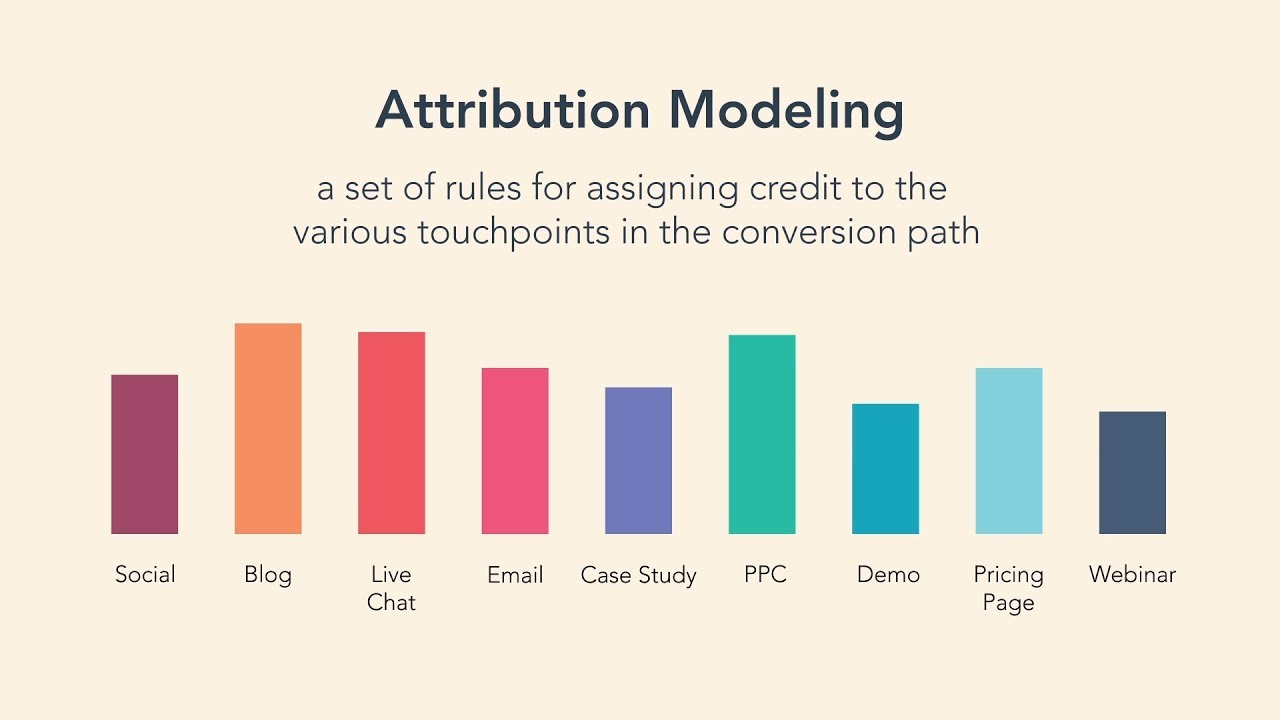
Attribution modeling
Attribution Modeling is also a tool to measure marketing efficiency, which is somehow bottom-side-up. According to theory, attribution modeling is when the conversion process is tracked and analyzed by checking out the data at all the steps included. It means that you can identify the value of each marketing initiative components by applying this modeling tool.
A long time ago, when eCommerce appeared and became more and more common, an unexpectedly large amount of data are captured and analyzed, which put huge pressure on marketers. To meet these requirements of eCommerce, attribution modeling was designed and applied with an attempt to focus on online sales, advertising, and other conversion efforts. Then, when marketers put more effort into mixing their online and offline channels to create good integration, attribution modeling was adjusted to include offline interactions that less easily yield their data.
Easily put, attribution modeling refers to the granular approach in which the data is analyzed very often, in real-time, or as close as is feasible. According to the size of the available data amount and the number of marketing channels in use, there are multiple types of attribution models. Each has its own goals, strengths, and weaknesses. Each has its own goals, strengths, and weaknesses. Here are some common types of attribution models:
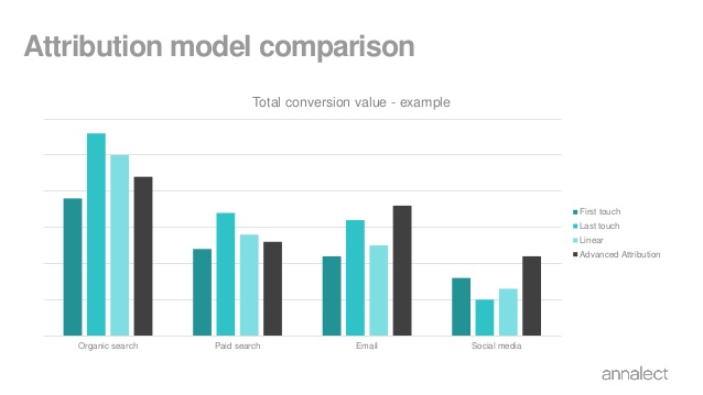
- Type 1: Last interaction attribution
This one is still a default method, and there are possible issues not considered when it comes to the last interaction attribution. This type is used in the first days of eCommerce when marketers gave all the credit for a conversion to the last lead users interacted with.
- Type 2: First interaction attribution
In this model, all the credit to the source of the user’s first impression of your business is taken into account.
- Type 3: Last non-direct click attribution
In terms of the last non-direct click model, it awards all credit to one interaction. It seems to be more advanced because it assumes all direct interactions should not get any credit. For example, when users visit your website directly by typing the URL. Nonetheless, this model means users remember that your site does exist due to exposure to previous marketing efforts.
- Type 4: Linear attribution
Being more innovative, the linear attribution model divides the credit equally among all interactions before conversion. However simple and fair it is, this model is sometimes not suitable because each interaction was not equally influential all the time.
- Type 5: Time decay attribution
This model can get over the weakness of the linear attribution model since it allows marketers to focus on the marketing pushes and convincing customers to close the deal. However, it still relies on some assumptions though.
- Type 6: U-shaped attribution (Position-Based attribution)
It is very reasonable since position-Based attribution spends 40% to the first interaction, 40% to the last interaction, and 20% to all the interactions appearing in-between. This seems to be suitable for most of the cases.
Differences between Marketing Mix Modeling and Attribution Modeling
As we mentioned very clearly above, MMM is designed in the retail sector to measure the efficiency of marketing activities and campaigns via TV, radio, print ads, or promotional efforts at the point of sale. When being compared with attribution modeling, MMM has some differences as follow:
-
Marketing mix modeling belittles real-time analysis but annual, biannual, or quarterly analysis based on aggregated historical data.
-
Marketing mix modeling focuses on a top-down, macro-level view instead of user interactions
-
Marketing mix modeling analyses sales data, revenue, benchmarks, costs, and outside factors (economic factors, market conditions, competitors, profit margins, and more)
The best model for your business
As you can see, the key difference between the two marketing modeling method is that Marketing Mix Modeling can deal with a wide range of data while Attribution Modeling does not.
Each model still has its strengths and weaknesses. Marketing mix modeling is a good option for almost every business because it provides:
-
A variety of marketing channels
-
More options for products as well as locations
-
Complex sets of marketing data to measure
-
An online and a brick-and-mortar presence
On the other hand, if your business is creating a simpler marketing strategy with relatively few marketing channels, attribution modeling is somehow more suitable. Being an easy analytic process, attribution modeling does not consider the impact of multiple concurrent marketing channels.
How does marketing mix modeling work?
MMM includes the “mix” factor because its target is mixing four key business elements (4P) in developing a company. Those elements are:
- Product: A tangible product or an intangible service that meets customers’ needs
- Price: An amount of money that customer is expected to pay for the product
- Place: The place in which companies sell their products and the way they are shipped to the market as well as the customers
- Promotion: Marketing communication strategies or channels in which marketing activities are taken such as advertising, offers, public relations, and more
They are mixed based on the data taken from all the factors that partly or totally impact the success of marketing channels and performing a regression analysis. According to theory, the line will show how each component of your marketing strategy affects your sales.
There are three types of factor deciding marketing mix which might include:
-
Incremental drivers: Incremental outcome is one produced by marketing activities such as digital spending, print advertising, TV advertising, price discounts, promotions, social outreach, and more.
-
Base drivers: On the other hand, base drivers mean those generated by activities that are out of advertisements. It is decided by the brand image and equity which is raised many years. If you can make sure there are no economic changes or environmental changes during this time, base outcomes can totally be fixed.
-
Other drivers: They are just sub-component of baseline factors but it does not mean this kind of driver is not essential. They are evaluated when the brand value increases over a period of time as a result of the long-term impact of marketing activities.
Therefore, the marketing mix model works to help you see how well all your marketing channels are working together.
Techniques used in marketing mix modeling
After gaining a deep insight into marketing mix modeling, now you must be wondering how to build an effective one, right? We are going to introduce the two most common techniques used in MMM to help you get started.
When it comes to marketing mix modeling, many marketers do not know how to build a good marketing mix model though they fully understand its importance. There are many techniques that have been applied in MMM. One of the most effective ones is known as ‘regression’ because it does well in measuring the most efficient mix of all marketing changes. Within regression, data is divided into two types which are dependent variables (DV) and independent variables (IDV). To handle this technique, marketers have to analyze how IDV impacts the outcome of DV. No matter how hard it is at the beginning, we can provide a correct estimation of the marketing mix on the business’s net profits.
Two most common marketing mix modeling regression techniques used are:
-
Linear regression
-
Multiplicative regression
Linear regression model
The Linear regression model is used when the dependent variables are endless and the distance between the dependent variables and independent variables tends to be narrow or linear. The mentioned relationship is made clear via the following equation:
y = β1 + β2X2 + β3X3 +…+βkXk + ε
As you can see from the equation, ‘y’ is the DV which is being estimated, Xs are the IDV and ε is the error term while βi’s are the regression coefficients. Y is the real outcome which is different from the predicted outcome y. This difference is called “a prediction error”.
The Linear regression model is applied in some cases such as:
-
Causal analysis: When marketers want to analyze the causes
-
Impact forecasting: When marketers want to predict how the changes impact
-
Trend forecasting: When marketers want to predict the following trends or future scenarios
Nonetheless, there’s still one minus point remaining which is its sensitivity to outliers, multicollinearity, and cross-correlation. Therefore, the Linear regression model is not chosen to deal with large amounts of data.
Multiplicative regression models
In the linear regression model or additive linear model, IDVs are simply added. It means it is a constant absolute effect of each additional unit of variables. Only when businesses are developed in a stable environment and there are no economic or environmental changes do they decide to apply the linear model. On the other hand, when the pricing is zero, the sales or dependent variables will be infinite.
Therefore, multiplicative regression models are designed to get over the disadvantages of the linear model. They present reality more realistically because IDVs are multiplied together. That’s why more marketers choose this kind of marketing mix modeling technique.
Why do we call ‘models’ instead of ‘model’? It is because there are two kinds of multiplicative regression techniques which are:
-
Semi-logarithmic models
-
Logarithmic models
Semi-logarithmic models
Semi-logarithmic models or Log-Linear models are when the exponents of independent variables are multiplied.
It is shown through the equation below:
Salest = exp (Intercept) * exp (β1Pricingt) exp (β2Distributiont) exp(β3Mediat) exp (β4Discountst) exp (β5Seasonalityt) exp (β6Promotionst) …
Or it can be written as:
Salest = exp (Intercept + β1Pricingt+ β2Distributiont+ β3Mediat+ β4Discountst+ β5Seasonalityt+ β6Promotionst+ …)
The additive model is when the logarithmic transformation of the target variable linearizes the model form. The difference between additive models and semi-logarithmic model is that DV is logarithmically transformed.
The equation of that is:
Ln (Salest) = Intercept + β1Pricingt+ β2Distributiont+ β3Mediat+ β4Discountst+ β5Seasonalityt+ β6Promotionst+ …
When using the semi-logarithmic model, marketers can get some following advantages:
The coefficients β can be interpreted as the % change in business outcome (sales) to a unit change in the IDVs.
Real-time scenarios are easier to predict and get closer since each IDV in the model form works on top of what has been already achieved by other drivers.
Logarithmic Models
This one is called Log-Log models, which means IDVs are subjected to the logarithmic transformation besides the target variable. You can follow the equation below:
Salest = exp (Intercept) * β1Pricingt β2Distributiont exp (β3Mediat) exp (β4Discountst) exp (β5Seasonalityt) exp (β6Promotionst) …
Or it can be rewritten in linear form as:
Ln (Salest) = Intercept + β1Ln (Pricingt)+ β2Ln (Distributiont)+ β3Mediat+ β4Discountst+ β5Seasonalityt+ β6Promotionst+ …
So, what is the difference between Log-Linear and Log-Log models? There is a variety but the main point bases on the interpretation of response coefficients. In this model, the coefficients are interpreted as the % change in business outcome (sales) in response to 1% change in the independent variable.
It means:
β = %ΔDependent_Variable / %ΔExplanatory_Variable
Constant elasticity of the target variable to explanatory variables is presented. When it comes to Log-Linear models, though it does not directly imply elasticity, it can be estimated via the coefficient as β · X every time. It increases in absolute value with the explanatory variable.
Related posts:
- How to use Google Trends?
- Aweber vs Mailchimp: Which One Should You Choose?
- Best Landing Page Builders
- Must-have eCommerce tools for Online Stores
Final thoughts
As you can see, marketing mix modeling is a useful technique that helps a company or business grow like wildflowers. It minimizes the danger associated with product launches or promotions as much as possible.
If you take the business environment seriously, it is essential that you create a comprehensive marketing mix model to ensure your company’s sustainable development. It will not only support your business strategy but also improve the profitability of your marketing initiatives. To develop a suitable marketing mix model for yourself, you need to have a complete understanding of this environment and the newest advanced marketing research methods.
We hope that this article is helpful to you. Let’s get started in building your correct marketing mix model to maximize your products or services’ performance and sales. Leave us a comment if you have any questions and follow us for more interesting posts.


New Posts


How To Set Up Google Analytics 4 For Your BigCommerce Store
